tidylinreg Example

The tidylinreg package fits a linear model to a dataset, and can be used to carry out regression. tidylinreg computes and returns a list of summary statistics of the coefficients of the fitted linear model, including standard error, test statistic, confidence interval, and p-value.

To use tidylinreg in a project:

from tidylinreg.tidylinreg import LinearModel

LinearModel

tidylinreg.tidylinreg.LinearModel

Data

To demonstrate Linear Regression using tidylinreg, we can use the California housing dataset. This dataset has 8 numeric, predictive attributes and the target.

Attributes:

• MedInc: median income in block group

• HouseAge: median house age in block group

• AveRooms: average number of rooms per household

• AveBedrms: average number of bedrooms per household

• Population: block group population

• AveOccup: average number of household members

• Latitude: block group latitude

• Longitude: block group longitude

Target: The target variable is the median house value for California districts, expressed in hundreds of thousands of dollars ($100,000).

from sklearn.datasets import fetch_california_housing
import pandas as pd

housing = fetch_california_housing(as_frame=True)
X = housing["data"]
y = housing["target"]

Train/Test Split

Make sure to split the data into train and test sets to avoid any violations of the Golden Rule!

from sklearn.model_selection import train_test_split

X_train, X_test, y_train, y_test = train_test_split(X, y, test_size=0.3, random_state=524)

EDA

EDA is not the focus of this example, so here’s just a quick preview of the data. A more detailed explanation of the data can be found here.

X_train

	MedInc	HouseAge	AveRooms	AveBedrms	Population	AveOccup	Latitude	Longitude
190	3.3750	52.0	4.011905	1.071429	647.0	3.851190	37.79	-122.24
19599	1.5500	17.0	5.425150	1.080838	672.0	2.011976	37.56	-120.93
20100	2.0057	52.0	5.061728	1.078189	609.0	2.506173	37.96	-120.23
9708	1.9385	28.0	3.600000	1.039252	1717.0	3.209346	36.67	-121.65
20518	1.9426	32.0	3.957935	1.072658	2046.0	3.912046	38.58	-121.56
...	...	...	...	...	...	...	...	...
19206	1.9932	29.0	4.329949	1.053299	990.0	2.512690	38.47	-122.72
15131	2.3693	11.0	4.434608	1.042254	1472.0	2.961771	32.86	-116.92
5652	2.1382	21.0	3.708333	1.058036	1699.0	2.528274	33.73	-118.29
12733	8.6572	20.0	8.130435	1.027174	1105.0	3.002717	38.58	-121.35
17402	2.2743	38.0	4.021419	1.062918	2601.0	3.481928	34.95	-120.44

14448 rows × 8 columns

Scaling

This model uses simple linear regression with no regularization, so scaling of the features is optional but not required. Scaling is useful if we are interested in comparing relative feature importance; however, we should keep the data in its original scale in this example so that the linear regression coefficient estimates are more interpretable.

# from sklearn.preprocessing import StandardScaler

# scaler = StandardScaler()
# X_train = pd.DataFrame(scaler.fit_transform(X_train),
#                        columns=X_train.columns,
#                        index=X_train.index)
# X_test = pd.DataFrame(scaler.fit_transform(X_test),
#                       columns=X_test.columns,
#                       index=X_test.index)

Fit

Let’s define our model and fit it to the training data!

Note:, we don’t need to add a column of ones to our data to get an intercept. The fit method takes care of this for you!

model = LinearModel()
model.fit(X_train, y_train)

Predict

How do our predictions look compared to the true values?

import matplotlib.pyplot as plt

preds = model.predict(X_test)

# Create a scatter plot
plt.scatter(y_test, preds, color='blue', label='Predictions')  # Scatter plot

# Add a reference line (y = x)
plt.plot([min(y_test), max(y_test)], [min(y_test), max(y_test)], 
         color='red', linestyle='--', label='Ideal Fit (y = x)')

# Add labels and title
plt.xlabel('True values')
plt.ylabel('Predictions')
plt.title('California Housing Predictions')
plt.legend()

# Display the plot
plt.grid(True)  # Optional: Add a grid for better readability
plt.show()

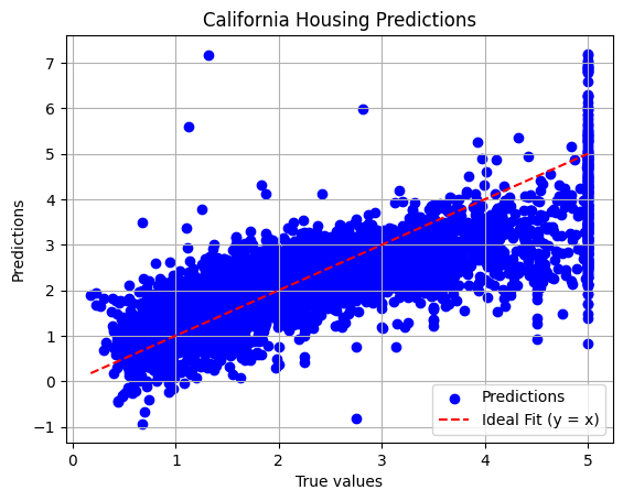
Our model is capturing the general trend of the data!

Summary Statistics

This is the great part of tidylinreg! Calling summary() will calculate important statistical values for the linear model coefficient estimates, including standard error, test statistic, confidence interval, and p-values. The output of summary() is generated by calling the following internal class methods:

• get_std_error()

• get_test_statistic()

• get_ci()

• get_pvalues()

model.summary()

	Parameter	Estimate	Std. Error	T-Statistic	P-Value
0	(Intercept)	-37.004147	0.790393	-46.817373	0.000000e+00
1	MedInc	0.438382	0.005039	86.989990	0.000000e+00
2	HouseAge	0.009267	0.000535	17.314654	0.000000e+00
3	AveRooms	-0.107089	0.006973	-15.358336	0.000000e+00
4	AveBedrms	0.635964	0.033466	19.003273	0.000000e+00
5	Population	-0.000007	0.000006	-1.160798	2.457431e-01
6	AveOccup	-0.003739	0.000536	-6.981016	3.058442e-12
7	Latitude	-0.422767	0.008629	-48.992423	0.000000e+00
8	Longitude	-0.435591	0.009039	-48.191074	0.000000e+00

As stated before, the intercept estimate was included without any need for modifying the dataframe.

Interpretations

Wow, it looks like all of our coefficient estimates are statistically significant, except for Population (with a significance level alpha = 0.05). We can also make interpretations on these statistically significant coefficients; for example, we can say that a unit increase in median income in the block group (MedInc) is associated with an increase of $43,838.20 in the median house value for the housing district (holding all other factors constant).

Lets look at another less intuitive example: We can see the AveOccup parameter has a statistically significant estimate of -0.003739. We can say that increasing the average occupancy by one person is associated to a decrease of $373.90 in the median house value for the housing district, while holding other factors constant.